Ensuring Data Integrity
Without ensuring data integrity, everything else is an exercise in futility.
By Greg Cenker
Greetings my fellow compatriots invested in quality assurance. This topic goes straight to the crux of any quality enriching process. No, we are not talking about Measurement Uncertainty Analysis (MU), Gage R&R, or Cpk. Before any of those methods come into play, the primary driver for any quality process is ensuring core data integrity. Without ensuring data integrity, everything else is an exercise in futility.
We are going to be dissecting six data integrity issues that require resolution prior to taking any further steps into the overall quality control process. These six points are:
Repeatability – does the data make sense and is it repeatable
Reproducibility – is the data reproducible
Resolution - The smallest increment an instrument can detect and display
Ramirez-Runger Test – does the data fit any distribution
IQR – (Interquartile Range) does the data contain outliers
ANOVA – (Analysis of Variance) does the data pass the F-Test
We will tackle the first two points, repeatability and reproducibility, in the opening segment.
Repeatability refers to the degree of mutual agreement among a series of individual measurements, values, or results with the same operator, measuring system, and procedure over a short period of time.
Reproducibility refers to the degree of mutual agreement among a series of individual measurements, values, or results with different operators, measuring systems, and/or procedures. An experiment is considered reproducible if it can replicate the results by anyone who properly follows the procedure.
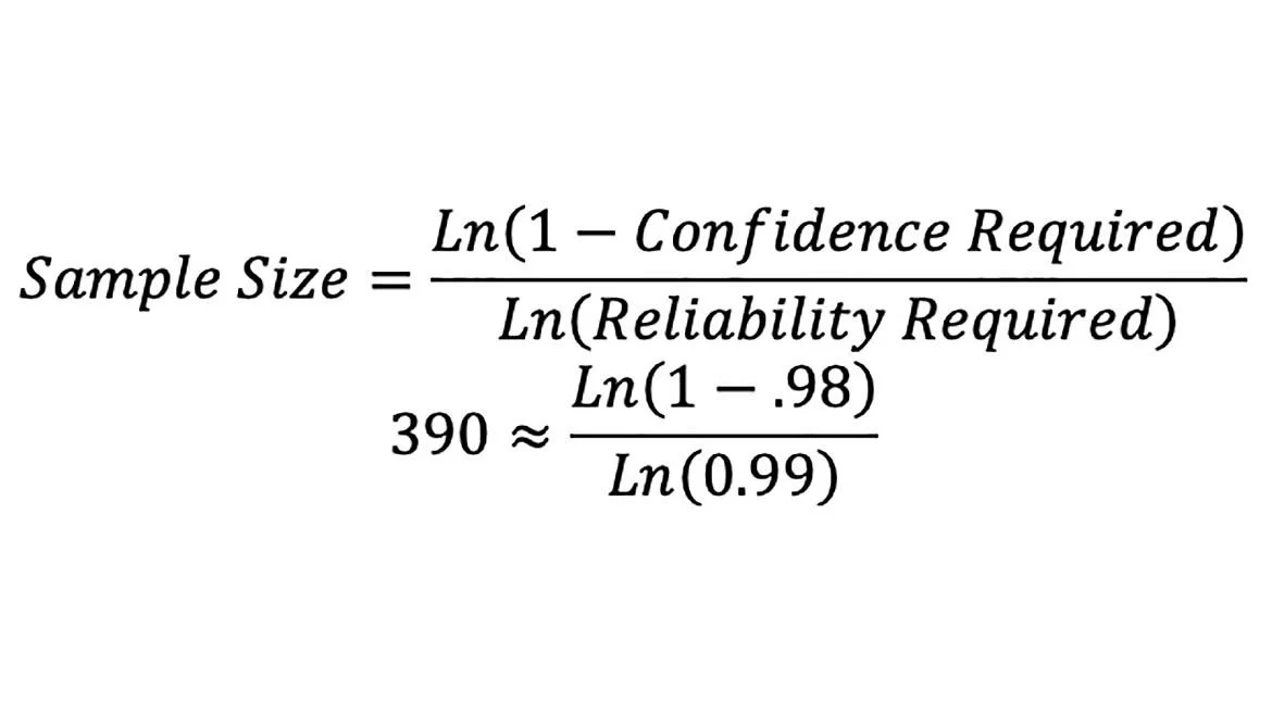
We want our reliability target to be 99% (1% risk) which should demonstrate 99% of the process data will meet the specification with at least 98% confidence. Sample size needed can be easily calculated by equation 1.
In this example, we are trying to qualify a measurement test system ensuring the process is repeatable and reproducible.
Gage R&R is not part of this exercise. It would be virtually impossible to assess Gage R&R using different manufactured Units Under Test (UUT’s) or Devices Under Test (DUT’s), when validating the testing system itself. Other elements of measurement uncertainty, although important, are outside the scope of this specific topic.
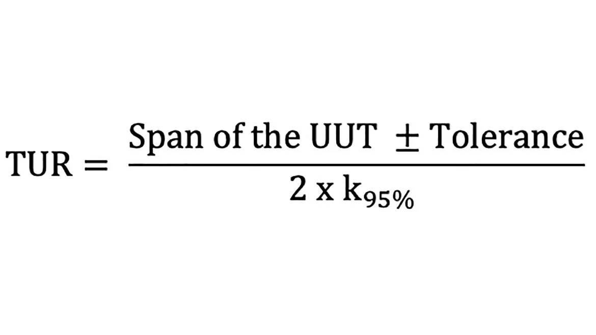
All measurements consist of a 6½ digit multimeter (DMM), within a testing fixture measuring a UUT or DUT, with the actual test point being +10 volts DC, ±10mVDC. The total uncertainty of the DMM itself is ±0.34 mVDC, providing a basic Test Uncertainty Ratio (TUR) >29:1 as shown in equation 2.
TUR is defined as the ratio of the span of the UUT (in this case 10.01 – 9.99 = 20mVDC) divided by 2 x k95%, where k95% = the expanded uncertainty of our DMM (this value is ±34 µVDC), which yields ~68µVDC (2 x 34µVDC). Note, this topic requires its own, separate article and is only mentioned in passing for proper context.
In preliminary testing we are utilizing the following criteria:
All measurement sequences are fully automated
The UUT was nominalized (i.e. set as close to +10V as possible) prior to commencement of the measurement sequence
There are three technicians performing the identical test
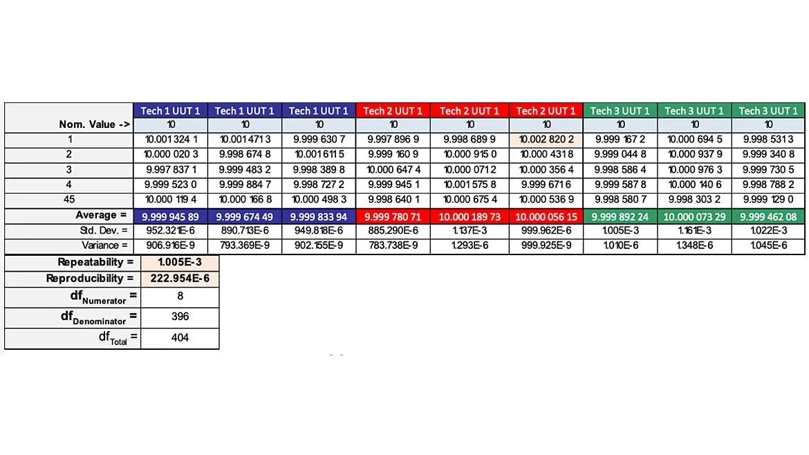
Each technician performs three, 45-point measurements on the same UUT (at +10 VDC). This provides 405 raw data points (remember, the minimum number required was 390). Basic statistics yield the following results (table 1 - abbreviated for demonstration purposes).
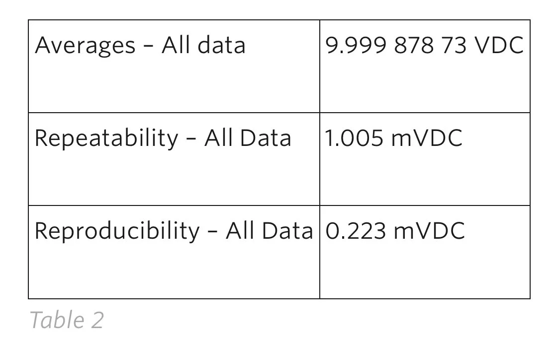
Through our initial testing, we observed the following numerical data (table 2):
Note: The mathematical calculations derived above will be shown later in this presentation.
The DMM uncertainty, UUT repeatability, and UUT reproducibility (corrected using effective degrees of freedom) account for a total of ~2.5mVDC which, overall, contributes less than 25% of the overall measurement process. Numerically this looks acceptable as a TUR >4:1, but is it as good as it could get?
Resolution
Resolution is the smallest increment an instrument can detect and display. For all the data collected, analyzed, and reported, it was mentioned that a 6½ digit multimeter (DMM) was utilized for the collection process. What was not mentioned was it was connected to a GPIB 488 bus utilizing software formatted to provide a maximum resolution of 7-digits. The problem, the DMM has a maximum usable resolution on the 10 VDC range of 1µVDC. The reported resolution from the GPIB buss was 0.1µVDC. In this case it wasn’t a serious cause for alarm. The reason for this mention is because I’ve seen test engineers complain about system “noise” while the instrument performing the measurement has a resolution of 1mV, yet they had their software configured to report 16 significant digits over the bus.
Ramirez – Runger Test
The following description is taken in part from a previously published article.
The Ramirez-Runger[1] test quantifies the chances that you can successfully fit any probability model to your data. By using this simple test to examine the assumptions behind all probability models, you can avoid making serious mistakes by selecting an inappropriate distribution model. The Ramirez-Runger test takes the time-order sequence of the data into account.
A probability model is an infinite sequence of random variables that are independent and identically distributed. And a sequence of independent and identically distributed random variables will display the same amount of variation regardless of whether the computation is carried out globally or sequentially. The Ramirez-Runger test compares a global estimate of dispersion with a sequential estimate.
The probability of exceedance, or p-value, for this test statistic quantifies how reasonable it is to consider the two estimates as being equivalent.
When they’re not equivalent, it’s unreasonable to assume that the data came from a sequence of independent and identically distributed random variables. When the data show evidence that they didn’t come from a sequence of independent and identically distributed random variables, the notion of a probability model vanishes. At this point, the probability of fitting a reasonable model to your data is nearly impossible.
This test, developed and published by Brenda Ramirez and George Runger in 2006, compares two different measures of dispersion. The first of these is the standard deviation statistic computed using all the data. The second of these is the average of the differences between successive values.
Using our collected data, we check for the probability we can sufficiently model it to a distribution.
[1] The Test to Use Before all Other Test- How to avoid mistakes in your analysis, Donald J Wheeler – April 30th, 2024
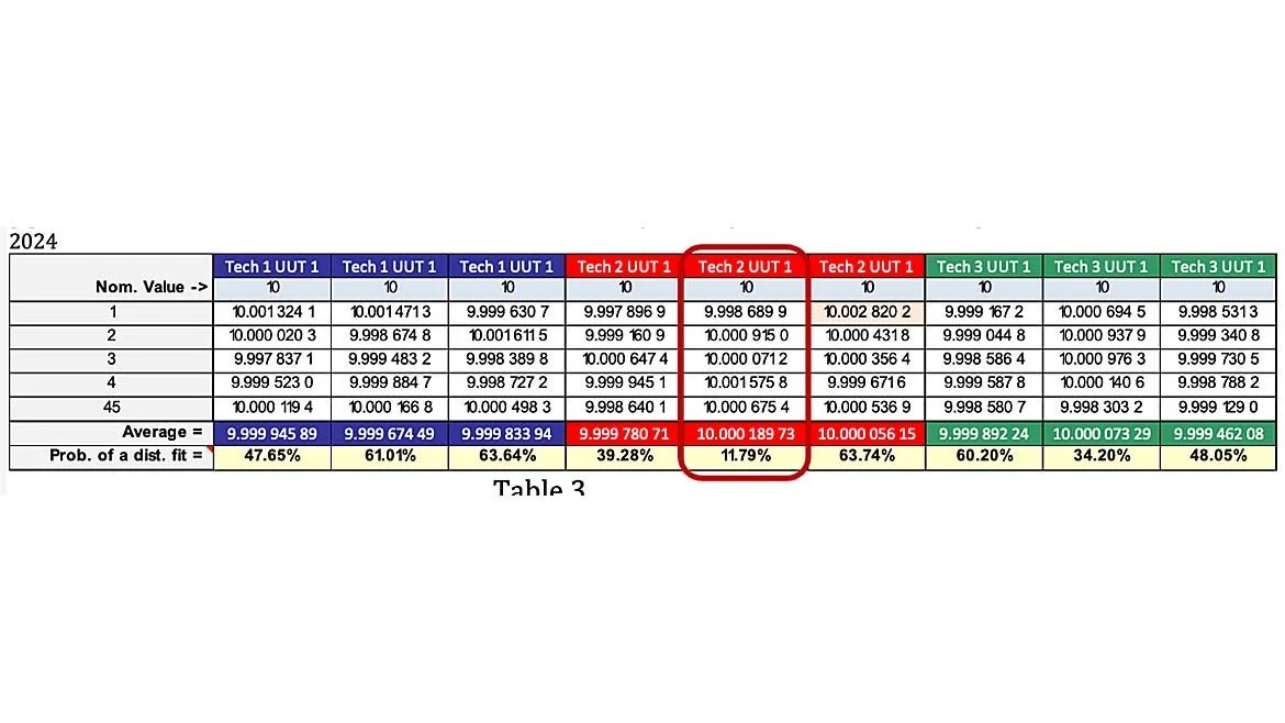
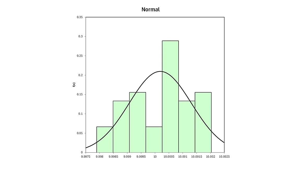
By using the Ramirez-Runger test, we can see that the worst probability fit comes from the data collected from Tech 2, on the 2nd 45-test point run of our UUT (table 3). This value shows there is a 11.79% probability of fitting a distribution model to the data. As a result, when we try to fit the data, the best fit determined with the data taken comes in the form of a normal distribution as shown in figure 1.
Although numerically and visually, this was the best fit, the graphic result isn’t very reassuring of a random, centrally distributed dataset.
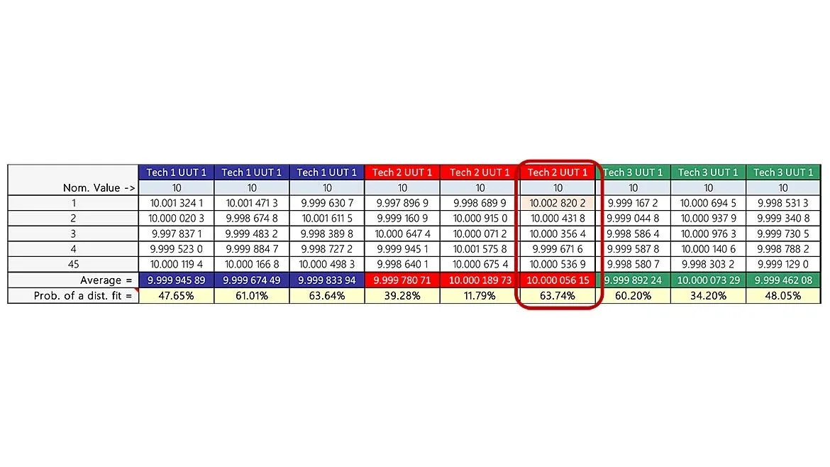
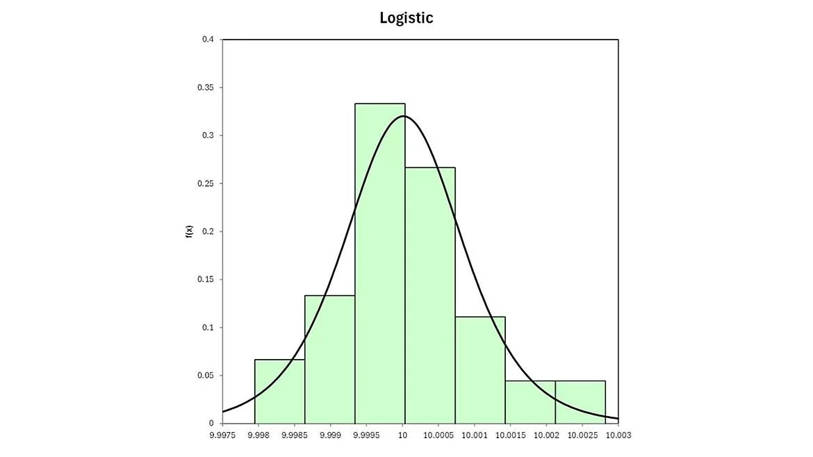
When referring to table 1 (reprise), and select the 3rd run from Tech 2, we see the probability of a distribution fit is nearly 64%
Moreover, the data suggests centrally dispersed random data as shown in figure 2.
Given the results of the distribution fit for data collected from Tech 2, run 2, it may be beneficial to re-run the data sequence again to either confirm or reject the finding of the poor fit and non-centrality.
IQR - Interquartile Range
The Interquartile Range (IQR)[2] measures the spread of the middle half of the dataset. It is the range for the middle 50% of your sampled data and will use the data itself to create boundaries that will either accept or reject any value falling outside the dataset with 99.25% confidence. In a nutshell, it constructs a statistical “fence” around your original dataset and any data collected residing outside this fence, is marked as an outlier (think of it as a ±acceptance tolerance). The difference is the value(s) may not be truly Out of Tolerance (OOT) with respect to the actual specification limits, however, points falling outside this range could be considered suspect.
Outliers are not necessarily bad; they are useful in identifying either rogue observations or displaying the true behavior of an instrument due to random variances.
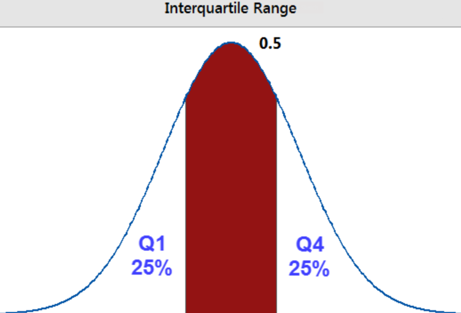
The interquartile range is the middle half of the data, it lies between the lower and upper quartiles and contains 50% of data points above Q1 and below Q4. The interquartile range graphically breaks up the dataset into 3 basic parts, ignoring any statistical distribution. The red portion of the graph below demonstrates the IQR (figure 3).
By utilizing this method, the combination creates a much fuller picture of the data distribution by centering it upon the median value.
The IQR method is very robust against outliers influencing the test results. The main reason for this efficiency is this method does not assume the data follow any distribution since the core function is centered around the median, not the mean value.
[2] Interquartile Range (IQR): How to Find and Use It, Statistics by Jim https://statisticsbyjim.com/basics/interquartile-range/
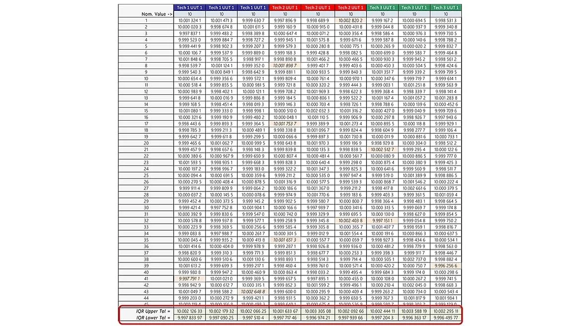
By applying this method to our sampled dataset, we can easily observe any values exceeding the 99.25% containment confidence bound. These values are shown as orange shaded cells as not complying (table 4).
The total process specification is ±10 mVDC, although all the data collected is still within expected specifications, it falls outside the IQR and are considered outliers.
ANOVA
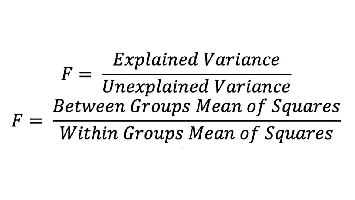
For our final qualifier, we will run ANOVA. ANOVA is a statistical method used to compare two or more data set averages to determine if the population means are equal. Essentially, the output of ANOVA helps assess whether there are significant differences between our measured groups. The two main functions in determining homogeneity are the F-Test and the significance test. The F-test is calculated as the ratio of explained variance to unexplained variance. Mathematically, in equation 3, it is written as:
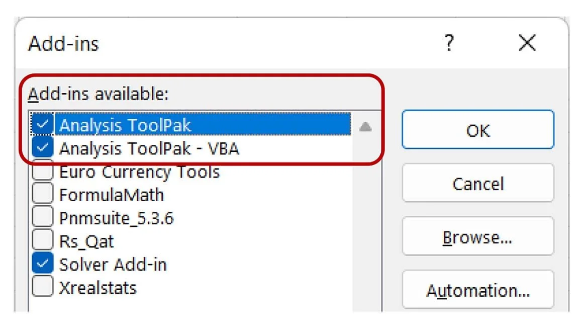
For simplicity, and readability of this article, the detailed mathematics explaining ANOVA are omitted however, creating ANOVA within Excel is a simple task. Firstly, ensure the option for Analysis ToolPak and Analysis ToolPak – VBA is checked in the developer menu (figure 4).
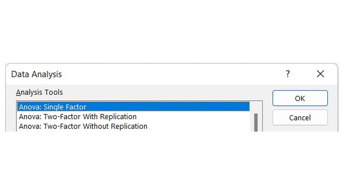
Once enabled, using the top menu selection, go to Data> Data Analysis (very far right of the menu selection)>Anova: Single Factor (figure 5).
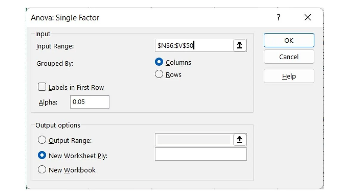
This action then brings up the following screen (figure 6). Simply select the data in the Input Range: field, leave Alpha: 0.05 (5% minimum), and for the Output options, use the radio button to select a new worksheet.
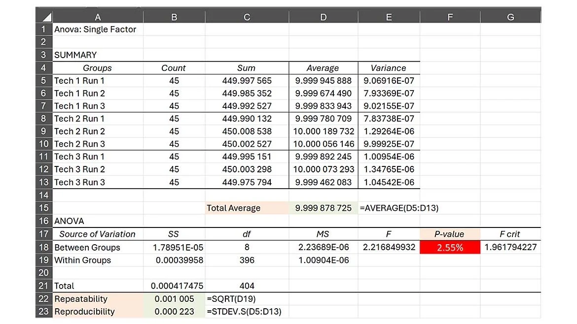
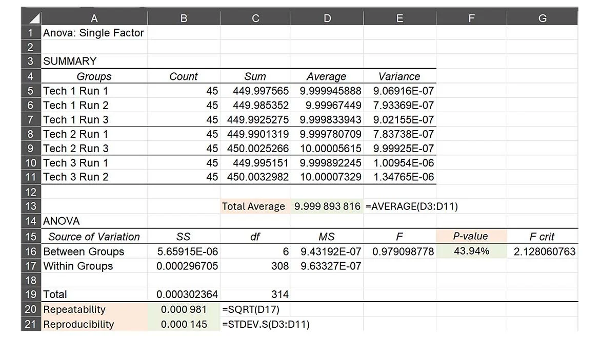
The output generated yields the following results (figure 7).
The “green” highlighted cell fields were added to the original ANOVA output to coincide calculated results of table 2 along with the mathematics behind the values. The results clearly show a “fail” as the significance test (P-value) reveals there is a 2.55% probability that the observed difference among the group means occurred by chance (our minimum was set to 0.05 or 5%). In essence, one can dismiss the assumption that all group means are equal, they are not.
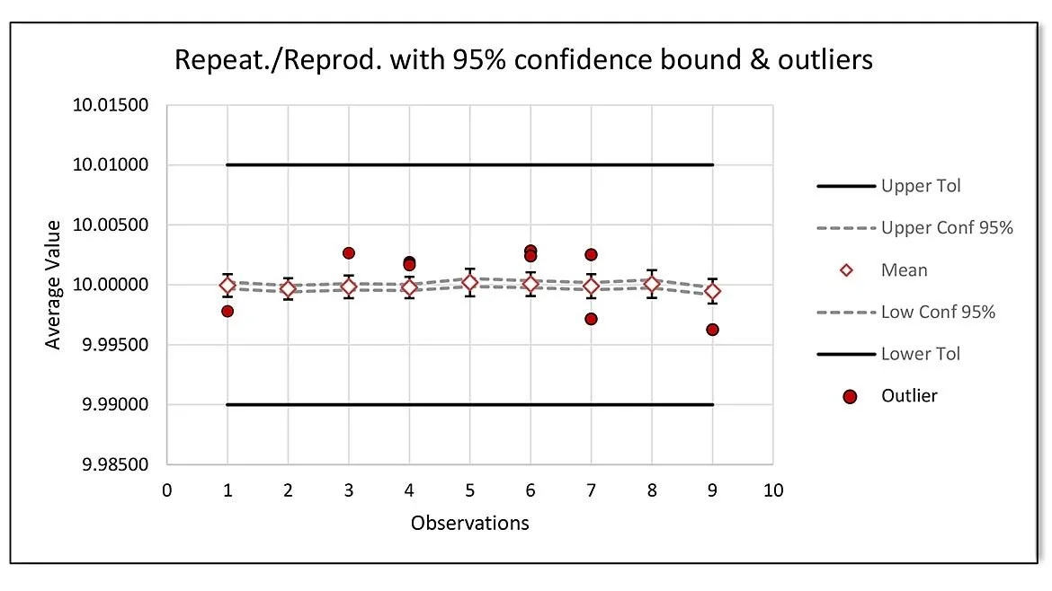
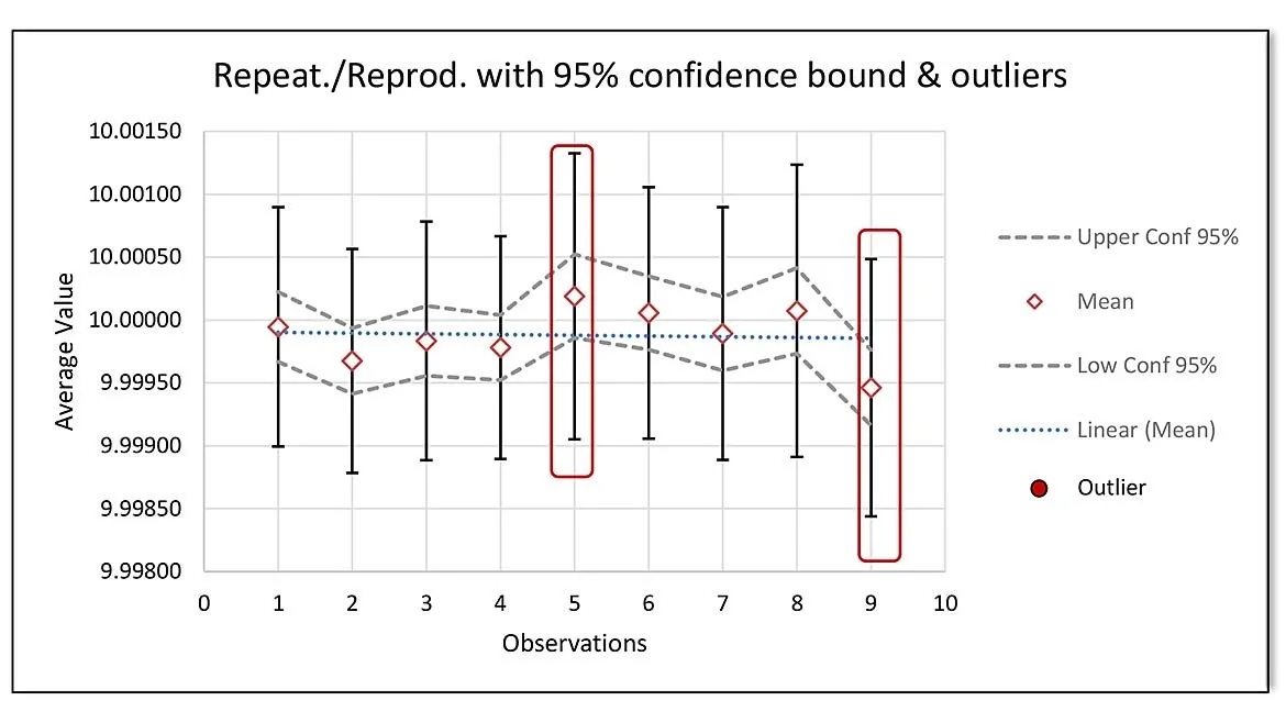
Although the numeric results are informative, a graphic of the dataset aids greatly in determining which runs may be suspect. All results were technically within specifications (figure 8), but upon zooming into the graphical data, the picture tells a different story (figure 9), observations 5 and 9 don’t belong as they are well outside the linear trend line estimate in figure 9.
To validate this hypothesis, observations 5 and 9 are omitted from ANOVA and the analysis is recalculated (figure 10)
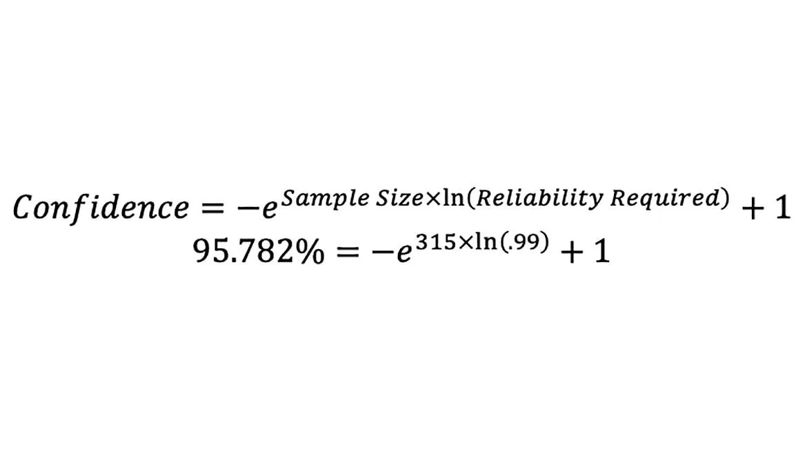
Now the process owner is faced with a dilemma, omit the two suspicious observation runs (5 and 9), or retest the same UUT again, with the same technicians originally performing the initial testing. If the data runs are omitted (leaving a total of 315 observations), the reliability target will remain at 99%, however, the confidence associated with that reliability value drops from ~98.293% to ~95.782% (equation 4).
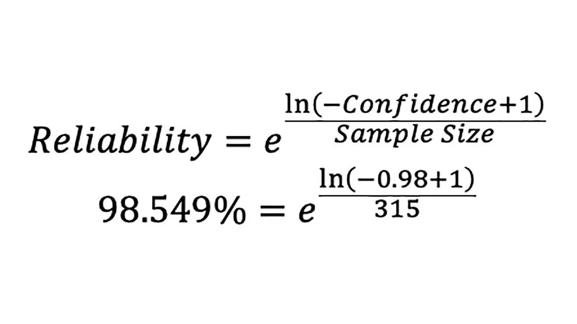
On the other hand, if confidence is to remain at 98%, reliability drops from 99% to 98.549% (equation 5).
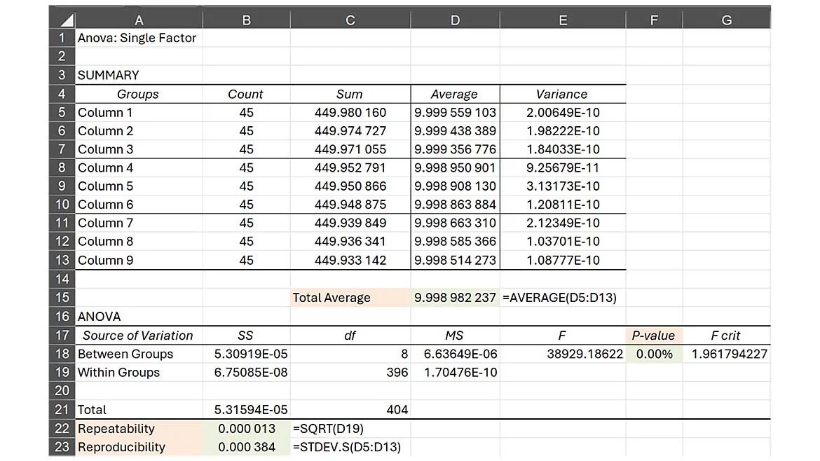
Although these differences are minor, in the following example, they can easily become significant, even when repeatability and reproducibility calculations are seemingly acceptable (figure 11).
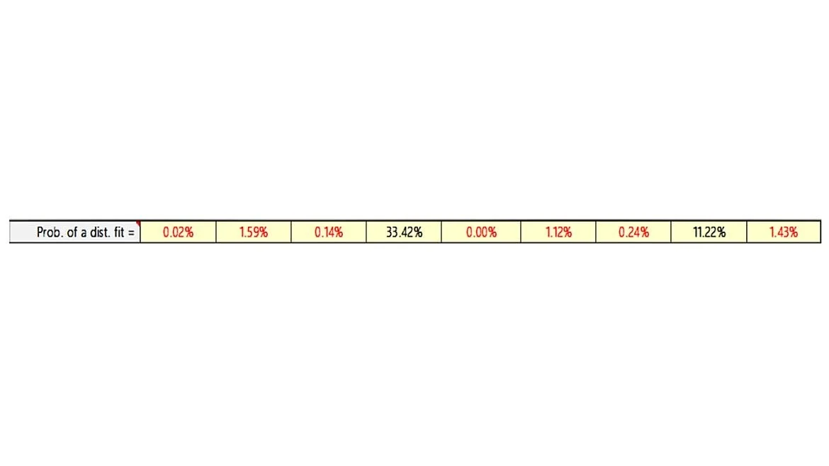
In this case, the repeatability and reproducibility are extremely small (13µVDC and 384µVDC respectively) however, the P-value is 0% meaning that the data is so incompatible with the null hypothesis, you can reject the entire population as being statistically equivalent. In addition, by running the Ramirez-Runger test, the data has near zero probability of fitting any distribution as shown in figure 12. The exception is run 4, but even that data point becomes questionable.
And finally, when the data is graphically visualized, it indicates a process that is not only unstable but out of control as well (figure 13).
Conclusion
Before one dives into uncertainty analysis, Gage R&R, Cpk, or other quality affecting metrics, often the simplest, and primary source of error, lies in the integrity of the data itself. Performing a repeatability and reproducibility evaluation may produce small errors, but they can easily mask underlying process anomalies which tend to cause significant heartburn downstream, at which time problems become much more expensive. In closing, we discussed the following and how, together, ensures the data taken is reliable and has veracity:
Repeatability – does the data make sense and is it repeatable
Reproducibility – is the data reproducible
Resolution - The smallest increment an instrument can detect and display
Ramirez-Runger Test – does the data fit any distribution
IQR – (Interquartile Range) does the data contain outliers
ANOVA – (Analysis of Variance) does the data pass the F-Test
These simple yet effective tools offer the process owner an accurate sanity check for data integrity long before a project gets the green light.
Greg Cenker is a senior metrologist for IndySoft, Daniel Island South Carolina.

