Understanding Filter and Outlier for CMM Application - Part 1
By Mark Boucher, CMM Quarterly
In this multi-part series, we will cover the general understanding of applying filters and which filters to apply.
Terminology
UPR
Undulations Per Revolution is a unit to describe how many times a wave occurs around a circumference in a given revolution. Circular features such as circles, cylinders, etc…should have the UPR filter type applied. When using a low pass filter, the higher the UPR the more harmonics we keep. The lower the UPR the more data is filtered or smoothed.
Choosing the correct UPR filter based on the bore size will divide the 360° bore by the UPR value. Shown here is the 15UPR to the bore diameter creating 15 sections. We will further explore how many points we need in each section.

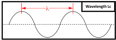
Wavelength
With cutoff wavelength you are choosing the size of the Gaussian filter that will be applied to every point. The higher the cutoff value the more smoothing or filtering occurs. This is the inverse of the UPR filter type.
Number of Points to Be Taken
There must be a minimum of 7 points per wavelength or undulation. If writing the program in Native DMIS change the value from 7 to 10 per the DMIS Standard.
Circular Features: A minimum of points equals the number of Undulations Per Revolution x 7.
o Ø8mm with 15UPR needs a minimum of 105 points. (15UPR x 7 points per undulation)
Linear Features: A minimum number of points equals the length x 7 points per wave/ Cutoff wavelength.
o Length of 100mm and a cutoff or 2.5 Lc needs a minimum or 280 points. (100mm in length x 7 points / 2.5)
Normal Distribution
Normal distribution: In filtering, it is important to consider the concept of normal distribution. Normal distribution describes how many measured points are located within dispersion width areas.

The normal distribution is a bell-shaped curve centered around the mean of a data set, and is divided by the sigma value, or standard deviation. The standard deviation is a measure used to quantify the amount of variation or dispersion in a data set. Approximately 68.27% of the data falls within ±1 standard deviation (σ) from the mean. Approximately 95.45% of the data lies within ±2 standard deviations, while approximately 99.73% falls within ±3 standard deviations. Data points beyond 3σ represent the remaining 0.27% of the data set and are typically considered outliers that may be excluded from analysis.

Low Pass Filter
When using a CMM, always apply the Low Pass filter if possible. This is crucial, especially with evaluation methods like minimum circumscribed or max inscribed, which rely on the extreme points of the data set. This filter allows low frequency data to pass through and ignores the roughness and waviness data found in higher frequencies. This shows the true form of the workpiece.
In Part 2 we will cover diametrical features.
